Computational Electromagnetics for Engineers
FDTD and FEM for RF structures, photonics, metamaterials, radar absorbers, and open-region scattering.
This page is organized around four things: governing equations, physical quantities with units, solver choice, and extraction of defensible observables.
Page focus
- Maxwell equations in usable engineering form
- Field, material, and observable quantities with SI units
- 1D to 2D progression for self-study
- Open-region modeling with source injection and CPML
Contents
1. Governing equations and physical quantities
Computational electromagnetics starts from Maxwell’s equations. The solver changes. The physics does not.
For linear isotropic media:
Use SI units unless a project convention states otherwise. In optics, wavelength is often reported in nm; in RF, frequency is often reported in MHz or GHz. The underlying SI units remain the reference.
Core field and material quantities
| Symbol | Name | SI unit |
|---|---|---|
| \(\mathbf{E}\) | Electric field | V/m |
| \(\mathbf{D}\) | Electric flux density | C/m² |
| \(\mathbf{H}\) | Magnetic field | A/m |
| \(\mathbf{B}\) | Magnetic flux density | T |
| \(\mathbf{J}\) | Current density | A/m² |
| \(\rho\) | Charge density | C/m³ |
| \(\varepsilon\) | Permittivity | F/m |
| \(\mu\) | Permeability | H/m |
| \(\sigma\) | Conductivity | S/m |
| \(\varepsilon_r\) | Relative permittivity | dimensionless |
| \(\mu_r\) | Relative permeability | dimensionless |
Wave and observable quantities
| Symbol | Name | SI unit |
|---|---|---|
| \(f\) | Frequency | Hz |
| \(\omega\) | Angular frequency | rad/s |
| \(\lambda\) | Wavelength | m |
| \(k_0\) | Free-space wavenumber | rad/m |
| \(\eta\) | Wave impedance | Ω |
| \(\mathbf{S}=\mathbf{E}\times\mathbf{H}\) | Poynting vector | W/m² |
| \(R\) | Reflectance | dimensionless or % |
| \(T\) | Transmittance | dimensionless or % |
| \(A\) | Absorptance | dimensionless or % |
| \(S_{11}, S_{12}, S_{21}, S_{22}\) | S-parameters | complex ratio; often magnitude, phase, or dB |
| \(Q\) | Quality factor | dimensionless |
FDTD in context. FDTD traces back to Yee’s 1966 staggered-grid formulation and became a practical mainstream tool after absorbing boundary treatments such as PML made open-region simulations reliable. Its historical strength is direct time-domain treatment of wave propagation, transients, and broadband scattering.
FEM in context. FEM grew out of variational and structural analysis methods and was established earlier in computational mechanics before becoming a standard electromagnetic tool. Its historical advantage is the weak-form framework, which naturally supports irregular geometries, boundary-value problems, and later multiphysics coupling.
2. Engineering observables
Use observables that connect directly to device performance.
Reflection / transmission
For slabs, coatings, filters, absorbers, and open-region scattering.
- \(R\): reflected power ratio. Unit: dimensionless or %.
- \(T\): transmitted power ratio. Unit: dimensionless or %.
- \(A\): absorbed power ratio. Unit: dimensionless or %.
S-parameters
For ports, feeds, antennas, RF packaging, and microwave components.
- \(S_{11}\): reflection seen at port 1. Unit: dimensionless complex ratio, often shown in dB.
- \(S_{21}\): transmission from port 1 to port 2. Unit: dimensionless complex ratio, often shown in dB.
- \(S_{12}\): transmission from port 2 to port 1. Unit: dimensionless complex ratio, often shown in dB.
- \(S_{22}\): reflection seen at port 2. Unit: dimensionless complex ratio, often shown in dB.
Field quantities
For hot spots, mode shape, localization, and power flow.
- \(\mathbf{E}\): electric field. Unit: V/m.
- \(\mathbf{H}\): magnetic field. Unit: A/m.
- \(|\mathbf{E}|^2\): electric-field intensity proxy. Unit: V²/m².
- \(|\mathbf{H}|^2\): magnetic-field intensity proxy. Unit: A²/m².
- \(\langle \mathbf{S} \rangle\): time-averaged power-flow density. Unit: W/m².
3. FDTD and FEM selection
| Method | Formulation | Main strength | Main limitation | Typical use |
|---|---|---|---|---|
| FDTD | Time domain, staggered grid | Broadband response from one pulse; good physical intuition | Time stepping cost; CFL limit; structured grid | Transient scattering, wideband spectra, source propagation |
| FEM | Frequency domain, weak form | Handles irregular geometry and boundary-value problems cleanly | Broadband response requires repeated frequency solves | Resonators, bounded domains, complex geometry, multiphysics coupling |
4. 1D finite-difference time-domain (FDTD)
5. 1D finite element method (FEM)
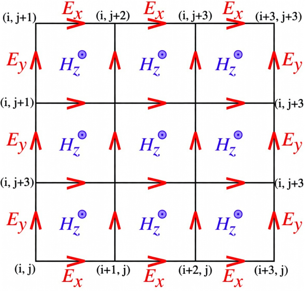
6. 2D finite-difference time-domain (FDTD)
7. 2D finite element method (FEM)
8. Workflow and validation
Before writing code or running a model, it is crucial to understand the overarching simulation pipeline. A rigorous workflow is the only way to prevent "garbage in, garbage out" and ensure your results represent reality.
The Standard Simulation Pipeline
Define Geometry & Materials
Set up the physical structure and critical length scales. Assign correct material properties (\(\varepsilon, \mu, \sigma\)) and verify unit conversions.
Select Discretization (Mesh)
Choose the appropriate solver (FDTD/FEM) and generate a grid or mesh that adequately resolves all structural features and wavelengths.
Apply Boundaries & Sources
Define how energy enters the system (ports, plane waves) and how the simulation edges behave. (This is heavily detailed in Section 9).
Solve & Extract Observables
Run the simulation and extract engineering observables (S-parameters, Reflectance) rather than relying solely on visual field plots.
Validation & Convergence
Ensure the extracted observables are independent of the mesh density and boundary distances.
Critical Checks
- Mesh refinement sensitivity.
- Time-step (CFL) limits for FDTD.
- Domain-size and boundary-distance sensitivity.
- Comparison against analytical reference models.
Common Failure Modes
- Under-resolved interfaces or curved geometry.
- Boundary reflection contaminating the answer.
- Wrong normalization of \(R\), \(T\), or S-parameters.
- Incorrect material data or unit scales.
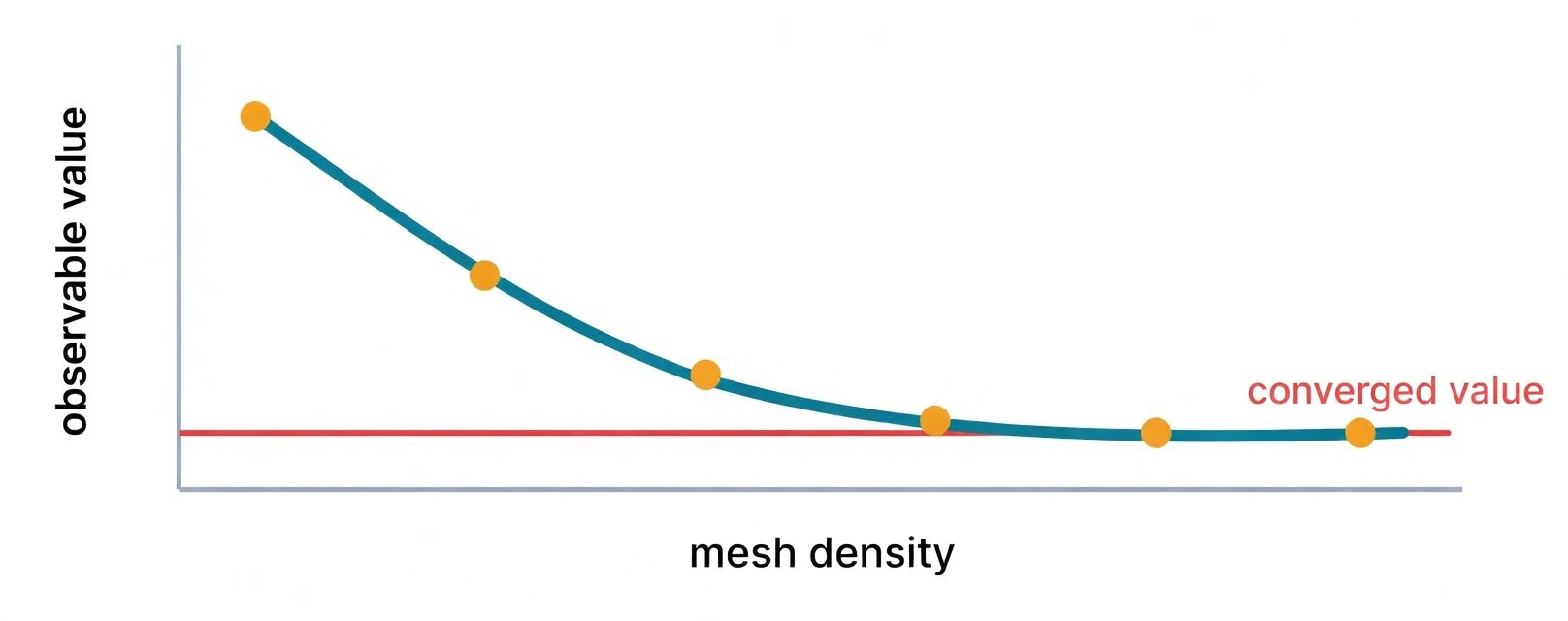
Use \(Q\) for any meaningful observable: reflected power, resonant frequency, transmission peak, or field energy. Convergence is defined on the observable, not on visual comfort.
As shown in the convergence curve, the observable value approaches a stable "converged value" as the mesh density increases. A proper mesh convergence check ensures that your computational results are grid-independent and physically defensible rather than an artifact of the discretization.
9. Sources and boundaries
Boundaries define the edges of your mathematical model and drastically influence accuracy. They are not a cosmetic implementation detail. The choice of boundary depends entirely on the physics of your problem.
Open Space / PML (Perfectly Matched Layer)
What it is: PML is an artificial absorbing sponge placed at the edges of the simulation domain to absorb outgoing waves without causing reflections.
When to use: Primarily used for modeling infinite free space, such as in scattering problems (e.g., radar cross-section, Mie scattering) or antenna propagation analysis.
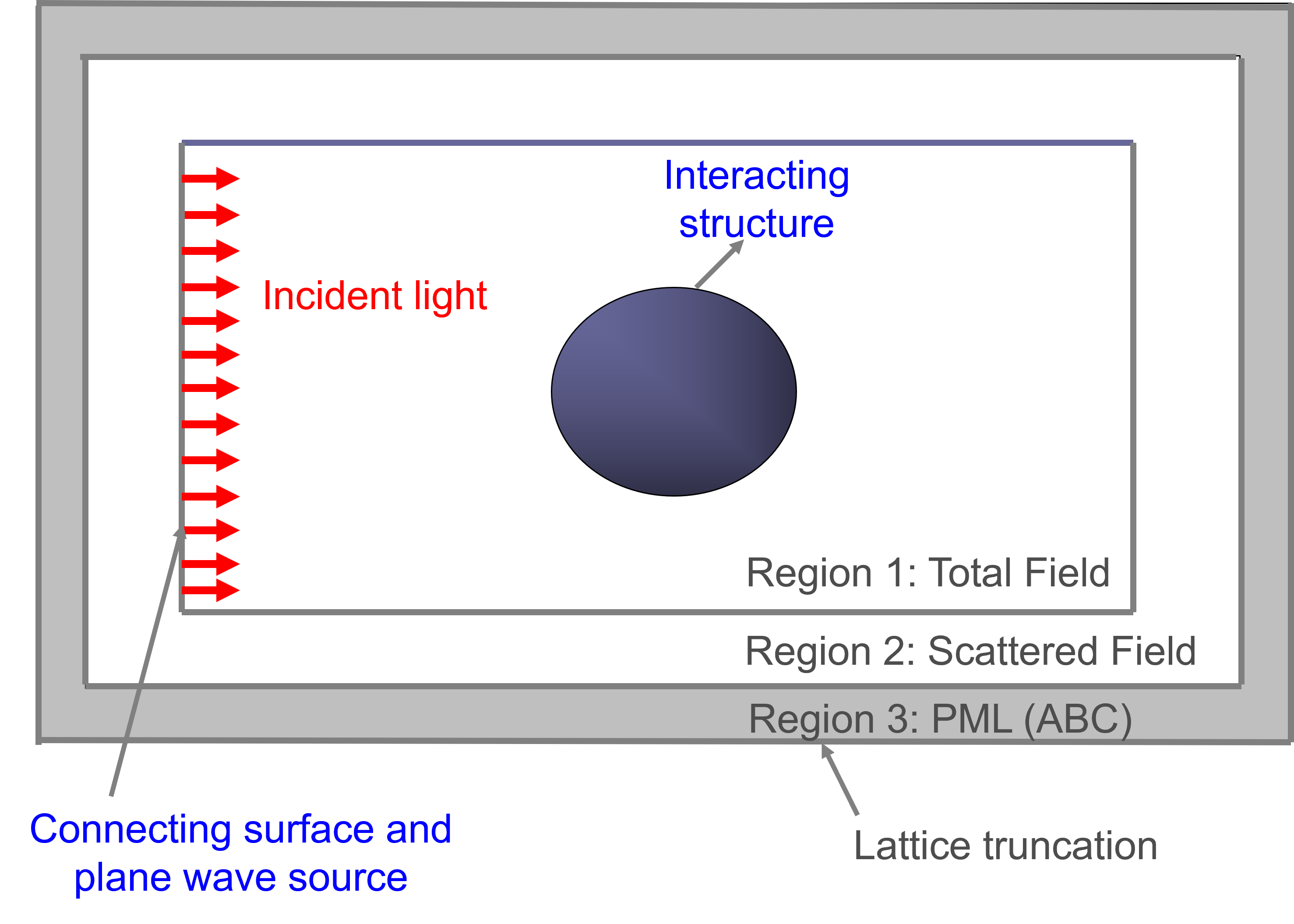
How to use: PMLs are often paired with a Total-Field Scattered-Field (TFSF) boundary. A plane wave is injected at the connecting surface. The innermost area (Region 1) calculates the total field (incident + scattered), while the outer area (Region 2) tracks only the scattered field before it is safely absorbed by the PML (Region 3).
Periodic Boundary Conditions (PBC)
What it is: PBCs wrap the fields from one side of the simulation domain to the opposite side, enforcing a periodic phase relationship.
When to use: Indispensable for modeling infinitely repeating structures such as metamaterials, frequency selective surfaces, and optical periodic gratings.
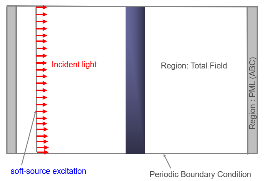
How to use: The simulation domain should cover exactly one unit cell of your structure. Apply a soft-source excitation to inject the wave. The transverse boundaries are set to PBC to maintain the infinite lateral extent, while the propagation axis is terminated with PML to absorb transmission and reflection.
Symmetry Boundaries (PEC / PMC)
Symmetry boundary conditions are optimization tools that can significantly reduce the required simulation volume and computation time by factors of 2, 4, or 8.
What it is: Perfect Electric Conductor (Symmetric) or Perfect Magnetic Conductor (Anti-Symmetric) boundaries force specific field components to zero along the plane of symmetry.
When to use: You can only use these when both the electromagnetic fields and the physical structure have a true plane of symmetry directly through the middle of the simulation region.
How to use: The correct option depends on your source polarization:
- If the source polarization is tangential to the plane of symmetry, select the symmetry option (PEC / Symmetric).
- If the source polarization is normal to the plane of symmetry, select the anti-symmetry option (PMC / Anti-Symmetric).
- No warnings for wrong settings: It is easy to accidentally select the wrong symmetry option. The software will not display a warning, but the simulation results will be completely incorrect. Always verify by running a full non-symmetric model first.
- Do not manually shrink the domain: Keep the original dimensions of the simulation region. If selected correctly, the solver will automatically shade the portion that isn't directly simulated and will automatically unfold the field data during analysis.
10. Example codes
1D FDTD slab
Gaussian pulse, dielectric slab, FFT-based \(R/T\) extraction.
1D FEM layered medium
Linear elements, piecewise \(\varepsilon\), sparse solve.
2D FDTD without ABC
Shows boundary reflection contamination in an open-region transient problem.
Suggested self-study path
- Reproduce \(R/T\) for a dielectric slab
- Add loss and compare \(A\)
- Move from ABC to CPML
- Compare FDTD and FEM on one shared structure
Selected engineering examples and validation notes
Finite-Difference Time-Domain (FDTD) Method
What this example demonstrates
Below I provide a two-dimensional TE FDTD implementation that includes:
- Yee-grid time stepping for TE polarization in 2D
- Total-field / scattered-field (TF/SF) formulation to inject an incident wave while separating scattered fields
- PML absorbing boundaries to approximate an open domain
The demonstration problem is electromagnetic scattering from a core–shell nanocylinder. The relative permittivities of the shell and core are set to 4 and 1, respectively. The simulation domain is divided into a total-field region, a scattered-field region, and surrounding PML layers. The animation visualizes the time evolution of the field (Ey) and provides an intuitive view of how the incident wave interacts with the core–shell structure and generates scattered waves.
The MATLAB implementation can be accessed here.
Notes on interpretation
- Why time-domain? In frequency-domain solvers you typically solve one frequency per run; in FDTD, a broadband pulse can reveal a wide spectral response from a single transient simulation.
- Why TF/SF? TF/SF allows clean separation between incident and scattered fields, which is particularly useful for scattering and extinction calculations.
- Why PML matters? Boundary reflections can contaminate scattering signatures; a properly configured PML reduces this artifact and improves the reliability of near- and far-field observables.
- Kane Yee (1966). “Numerical solution of initial boundary value problems involving Maxwell's equations in isotropic media”. IEEE Transactions on Antennas and Propagation, 14(3), 302–307.
- Allen Taflove and Susan C. Hagness (2005). Computational Electrodynamics: The Finite-Difference Time-Domain Method, 3rd ed. Artech House Publishers. ISBN 978-1-58053-832-9.
Plasmonic Metal Nanoparticles
Over the last two decades, plasmon resonances in metallic nanoparticles have been studied extensively because metallic nanostructures can strongly absorb and scatter light through localized surface plasmon resonances. This behavior underpins a broad range of applications, including optical sensing, photothermal heating and solar vapor generation, and bio-imaging.
Here I provide a 2D-TE FDTD code to compute extinction, scattering, and absorption efficiencies for a gold-shell dielectric-core nanocylinder. The Fortran implementation can be accessed here.
Analytical benchmark for verification
For 2D scattering problems with cylindrical symmetry, it is valuable to have an analytical solution as a reference for verifying numerical results. For this reason, I also provide an analytical code to calculate the extinction spectrum of a core–shell nanocylinder. As an example, results for a gold-shell dielectric-core nanocylinder with outer radius 50 nm and inner radius 40 nm are compared against the corresponding FDTD simulations in the figure below. The analytical implementation can be accessed here.
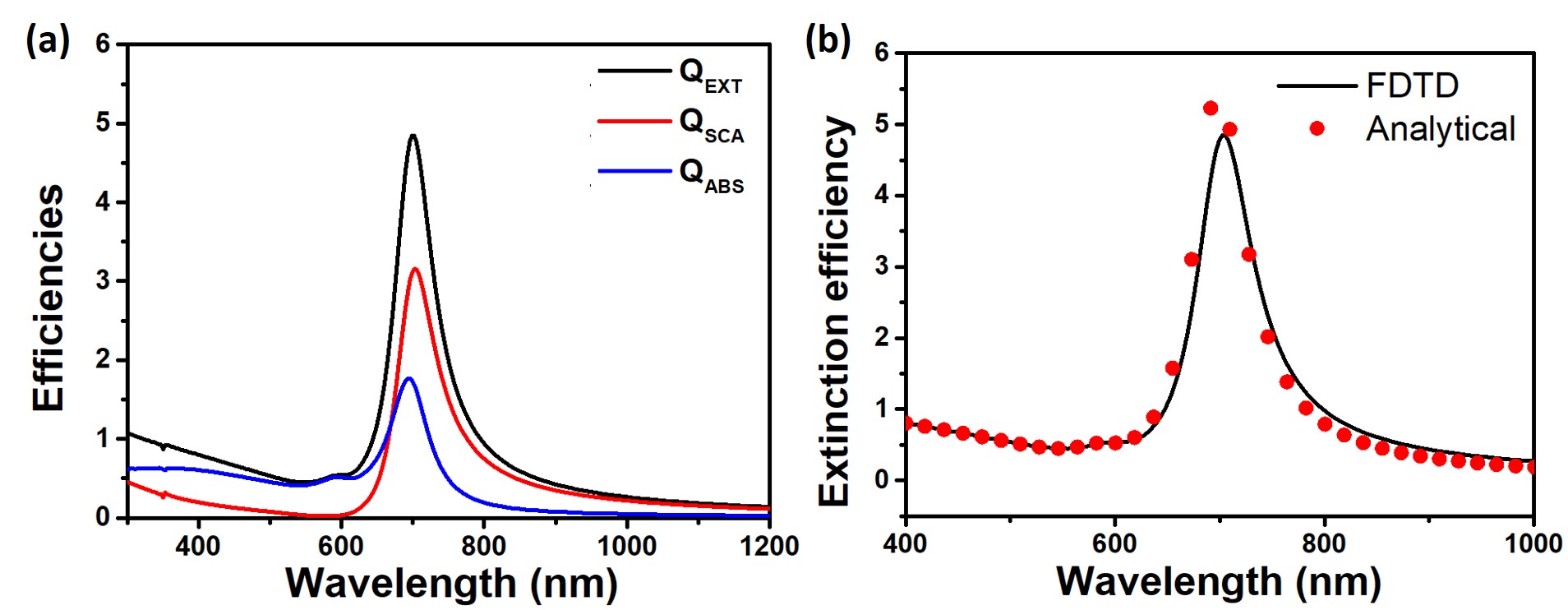
- Why this comparison is useful: matching peak positions and spectral trends provides a practical sanity check on discretization, TF/SF injection, and boundary absorption settings.
- What can differ: small deviations may arise from finite grid resolution, numerical dispersion, PML configuration, and the time-window / Fourier-transform settings used to extract spectra from transient fields.